k近邻算法
原理
存在一个样本数据集合,也称作训练样本集,且我们知道样本中每个数据的分类信息。
当我们输入未分类的新数据后,得到新数据与每个样本数据之间的”距离”,选择前k个距离
最近的样本中类别出现次数最多者作为新数据的类别
- 优点:精度高、对异常值不敏感、无数据输入假定
- 缺点:计算复杂度高、空间复杂度高
- 适用数据范围:数值型和标称型
示例
假设我们有如下样本集
| 电影名称 | 打斗镜头 | 接吻镜头 | 电影类型 |
|---|---|---|---|
| California Man | 3 | 104 | 爱情片 |
| He’s Not Really into Dudes | 2 | 100 | 爱情片 |
| Beautiful Woman | 1 | 81 | 爱情片 |
| Kevin Longblade | 101 | 10 | 动作片 |
| Robo Slayer 3000 | 99 | 5 | 动作片 |
| Amped 2 | 98 | 2 | 动作片 |
| ? | 18 | 90 | 未知 |
即便我们不知道未知电影的类型,我们也可以计算出来。首先得到未知电影与已知数据之间的距离:
| 电影名称 | 与未知电影的距离 |
|---|---|
| California Man | 20.5 |
| He’s Not Really into Dudes | 18.7 |
| Beautiful Woman | 19.2 |
| Kevin Longblade | 115.3 |
| Robo Slayer 3000 | 117.4 |
| Amped 2 | 118.9 |
现在可以找到k个距离最近的电影,取k=3,则可发现这三个电影均为爱情片,所以可以判断该电影为爱情片。
knn算法的步骤
- 计算已知类别数据集中的点与当前点之间的距离;
- 按照距离递增次序排序;
- 选取与当前点距离最小的k个点;
- 确定前k个点所在类别的出现频率;
- 返回前k个点出现频率最高的类别作为当前点的预测分类。
代码实现
1 | from numpy import tile, operator |
示例:使用k近邻算法改进约会网站的配对效果
数据
| 每年飞行常客里程数 | 玩视频游戏所耗时间百分比 | 每周消费冰激凌公升数 | 吸引力类型 |
|---|---|---|---|
| 40920 | 8.32697 | 0.953952 | largeDoses |
| 14488 | 7.153469 | 1.673904 | smallDoses |
| … | … | … | … |
解析数据
1 | def file2matrix(filename): |
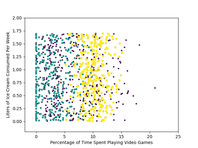
分析数据:绘图
安装matplotlib
1 | pip install matplotlibrc |
绘图
1 | plt.figure() |
数据归一化
数据中不同的属性之间量程相差很大,需要对数据进行归一化处理,常用的
归一化公式为:
1 | newValue = (oldValue-min)/(max-min) |
实现代码:
1 | def autoNorm(dataSet): |
测试算法
1 | def datingClassTest(): |
在测试数据为50%的情况下,得到了6.4%的误差率,分类效果还可以。
完善分类器的应用
接下来就是利用该分类器来对数据进行分类了,即判断约会对象的吸引力:
1 | def classifyPerson(): |
实例:手写识别系统
为简单起见,这里只处理0-9的数字。原始图像经过处理后,得到如下所示的数据:
1 | 00000000000001100000000000000000 |
上图是数字0的二维数据(32*32),需要先转为1*1024的数据才能使用前面的分类算法。
1 | def img2vector(filename): |
接下来,测试分类器的分类效果:
1 | def handwritingClassTest(): |
小结
上述代码稍微运行了一会才出来结果,因为需要对每个测试向量计算2000次距离计算,包括1024个浮点运算,比较耗时。
另外,如果训练数据很大,需要使用大量的存储空间。
k近邻算法的另外一个缺陷是它无法给出任何数据的基础结构信息,因此也无法知晓平均实例样本和典型实例样本具有什么特征。